📝 Guest Post: Yandex develops and open-sources YaFSDP — a tool for faster LLM training and optimized GPU consumption*

A few weeks ago, Yandex open-sourced the YaFSDP method — a new tool that is designed to dramatically speed up the training of large language models. In this article, Mikhail Khrushchev, the leader of the YandexGPT pre-training team will talk about how you can organize LLM training on a cluster and what issues may arise. He’ll also look at alternative training methods like ZeRO and FSDP and explain how YaFSDP differs from them.

Problems with Training on Multiple GPUs

What are the challenges of distributed LLM training on a cluster with multiple GPUs? To answer this question, let’s first consider training on a single GPU:

1. We do a forward pass through the network for a new data batch and then calculate loss.

2. Then we run backpropagation.

3. The optimizer updates the optimizer states and model weights.

So what changes when we use multiple GPUs? Let’s look at the most straightforward implementation of distributed training on four GPUs (Distributed Data Parallelism):

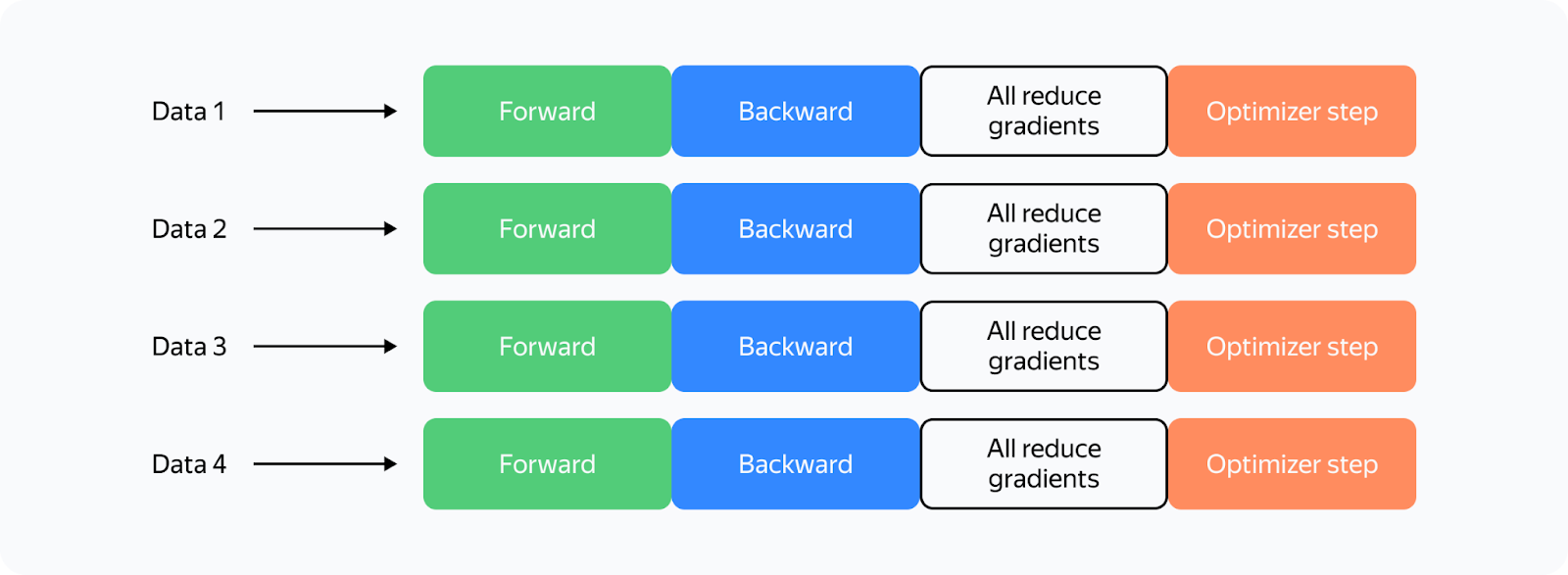
What’s changed? Now:

1. Each GPU processes its own chunk of a larger data batch, allowing us to increase the batch size fourfold with the same memory load.

2. We need to synchronize the GPUs. To do this, we average gradients among GPUs using all_reduce to ensure the weights on different maps are updated synchronously. The all_reduce operation is one of the fastest ways to implement this: it’s available in the NCCL (NVIDIA Collective Communications Library) and supported in the torch.distributed package.

Let’s recall the different communication operations (they are referenced throughout the article):

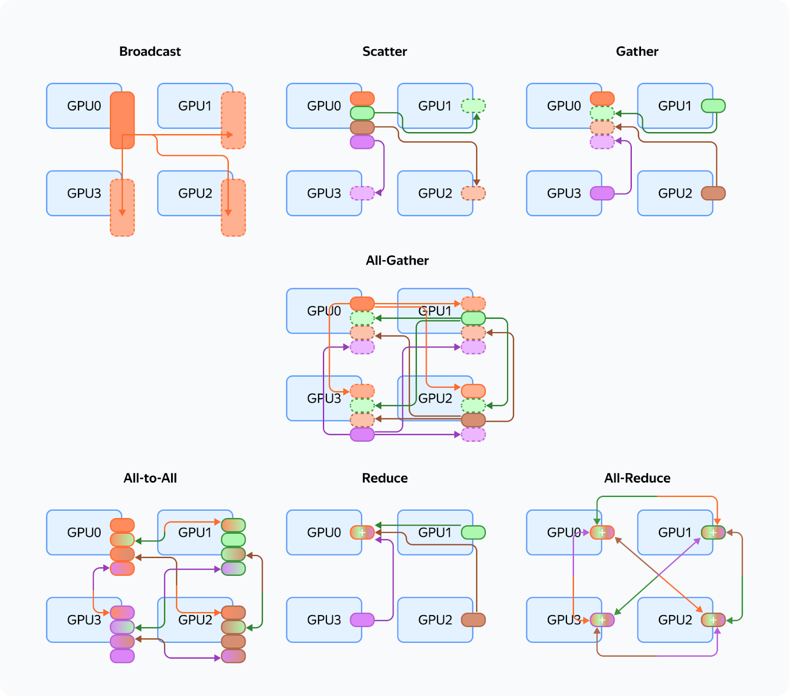
These are the issues we encounter with those communications:

1. In all_reduce operations, we send twice as many gradients as there are network parameters. For example, when summing up gradients in fp16 for Llama 70B, we need to send 280 GB of data per iteration between maps. In today’s clusters, this takes quite a lot of time.

2. Weights, gradients, and optimizer states are duplicated among maps. In mixed precision training, the Llama 70B and the Adam optimizer require over 1 TB of memory, while a regular GPU memory is only 80 GB.

This means the redundant memory load is so massive we can’t even fit a relatively small model into GPU memory, and our training process is severely slowed down due to all these additional operations.

Is there a way to solve these issues? Yes, there are some solutions. Among them, we distinguish a group of Data Parallelism methods that allow full sharding of weights, gradients, and optimizer states. There are three such methods available for Torch: ZeRO, FSDP, and Yandex’s YaFSDP.

ZeRO

In 2019, Microsoft’s DeepSpeed development team published the article ZeRO: Memory Optimizations Toward Training Trillion Parameter Models. The researchers introduced a new memory optimization solution, Zero Redundancy Optimizer (ZeRO), capable of fully partitioning weights, gradients, and optimizer states across all GPUs:

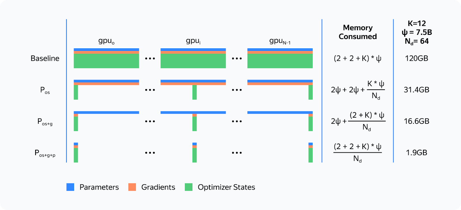
The proposed partitioning is only virtual. During the forward and backward passes, the model processes all parameters as if the data hasn’t been partitioned. The approach that makes this possible is asynchronous gathering of parameters.

Here’s how ZeRO is implemented in the DeepSpeed library when training on the N number of GPUs:

1. Each parameter is split into N parts, and each part is stored in a separate process memory.

2. We record the order in which parameters are used during the first iteration, before the optimizer step.

3. We allocate space for the collected parameters. During each subsequent forward and backward pass, we load parameters asynchronously via all_gather. When a particular module completes its work, we free up memory for this module’s parameters and start loading the next parameters. Computations run in parallel.

4. During the backward pass, we run reduce_scatter as soon as gradients are calculated.

5. During the optimizer step, we update only those weights and optimizer parameters that belong to the particular GPU. Incidentally, this speeds up the optimizer step N times!

Here’s how the forward pass would work in ZeRO if we had only one parameter tensor per layer:

The training scheme for a single GPU would look like this:

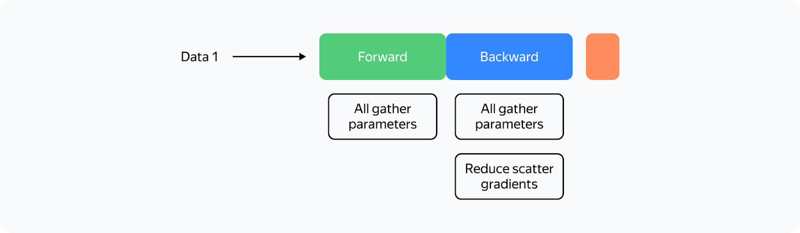
From the diagram, you can see that:

1. Communications are now asynchronous. If communications are faster than computations, they don’t interfere with computations or slow down the whole process.

2. There are now a lot more communications.

3. The optimizer step takes far less time.

The ZeRO concept implemented in DeepSpeed accelerated the training process for many LLMs, significantly optimizing memory consumption. However, there are some downsides as well:

1. Many bugs and bottlenecks in the DeepSpeed code.

2. Ineffective communication on large clusters.

A peculiar principle applies to all collective operations in the NCCL: the less data sent at a time, the less efficient the communications.

Suppose we have N GPUs. Then for all_gather operations, we’ll be able to send no more than 1/N of the total number of parameters at a time. When N is increased, communication efficiency drops.

In DeepSpeed, we run all_gather and reduce_scatter operations for each parameter tensor. In Llama 70B, the regular size of a parameter tensor is 8192 × 8192. So when training on 1024 maps, we can’t send more than 128 KB at a time, which means network utilization is ineffective.

• DeepSpeed tried to solve this issue by simultaneously integrating a large number of tensors. Unfortunately, this approach causes many slow GPU memory operations or requires custom implementation of all communications.

As a result, the profile looks something like this (stream 7 represents computations, stream 24 is communications):

Evidently, at increased cluster sizes, DeepSpeed tended to significantly slow down the training process. Is there a better strategy then? In fact, there is one.

The FSDP Era

The Fully Sharded Data Parallelism (FSDP), which now comes built-in with Torch, enjoys active support and is popular with developers.

What’s so great about this new approach? Here are the advantages:

1. FSDP combines multiple layer parameters into a single FlatParameter that gets split during sharding. This allows for running fast collective communications while sending large volumes of data.

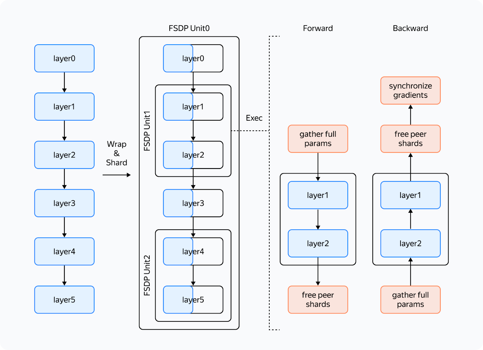
Based on an illustration from the FSDP documentation

2. FSDP has a more user-friendly interface:
   — DeepSpeed transforms the entire training pipeline, changing the model and optimizer.
   — FSDP transforms only the model and sends only the weights and gradients hosted by the process to the optimizer. Because of this, it’s possible to use a custom optimizer without additional setup.

3. FSDP doesn’t generate as many bugs as DeepSpeed, at least in common use cases.

4. Dynamic graphs: ZeRO requires that modules are always called in a strictly defined order, otherwise it won’t understand which parameter to load and when. In FSDP, you can use dynamic graphs.

Despite all these advantages, there are also issues that we faced:

1. FSDP dynamically allocates memory for layers and sometimes requires much more memory than is actually necessary.

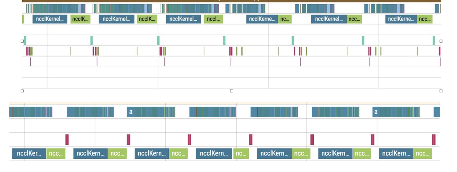
2. During backward passes, we came across a phenomenon that we called the “give-way effect”. The profile below illustrates it:

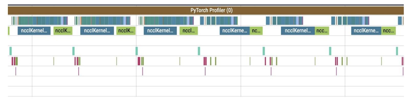
The first line here is the computation stream, and the other lines represent communication streams. We’ll talk about what streams are a little later. 

So what’s happening in the profile? Before the reduce_scatter operation (blue), there are many preparatory computations (small operations under the communications). The small computations run in parallel with the main computation stream, severely slowing down communications. This results in large gaps between communications, and consequently, the same gaps occur in the computation stream.

We tried to overcome these issues, and the solution we’ve come up with is the YaFSDP method.

YaFSDP

In this part, we’ll discuss our development process, delving a bit into how solutions like this can be devised and implemented. There are lots of code references ahead. Keep reading if you want to learn about advanced ways to use Torch.

So the goal we set before ourselves was to ensure that memory consumption is optimized and nothing slows down communications.

Why Save Memory?

That’s a great question. Let’s see what consumes memory during training:

— Weights, gradients, and optimizer states all depend on the number of processes and the amount of memory consumed tends to near zero as the number of processes increases.
— Buffers consume constant memory only.
— Activations depend on the model size and the number of tokens per process.

It turns out that activations are the only thing taking up memory. And that’s no mistake! For Llama 2 70B with a batch of 8192 tokens and Flash 2, activation storage takes over 110 GB (the number can be significantly reduced, but this is a whole different story).

Activation checkpointing can seriously reduce memory load: for forward passes, we only store activations between transformer blocks, and for backward passes, we recompute them. This saves a lot of memory: you’ll only need 5 GB to store activations. The problem is that the redundant computations take up 25% of the entire training time.

That’s why it makes sense to free up memory to avoid activation checkpointing for as many layers as possible.

In addition, if you have some free memory, efficiency of some communications can be improved.

Buffers

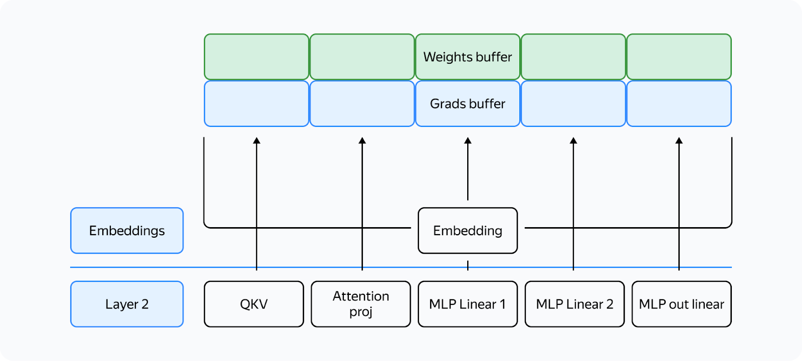
Like FSDP, we decided to shard layers instead of individual parameters — this way, we can maintain efficient communications and avoid duplicate operations. To control memory consumption, we allocated buffers for all required data in advance because we didn’t want the Torch allocator to manage the process. 

Here’s how it works: two buffers are allocated for storing intermediate weights and gradients. Each odd layer uses the first buffer, and each even layer uses the second buffer.

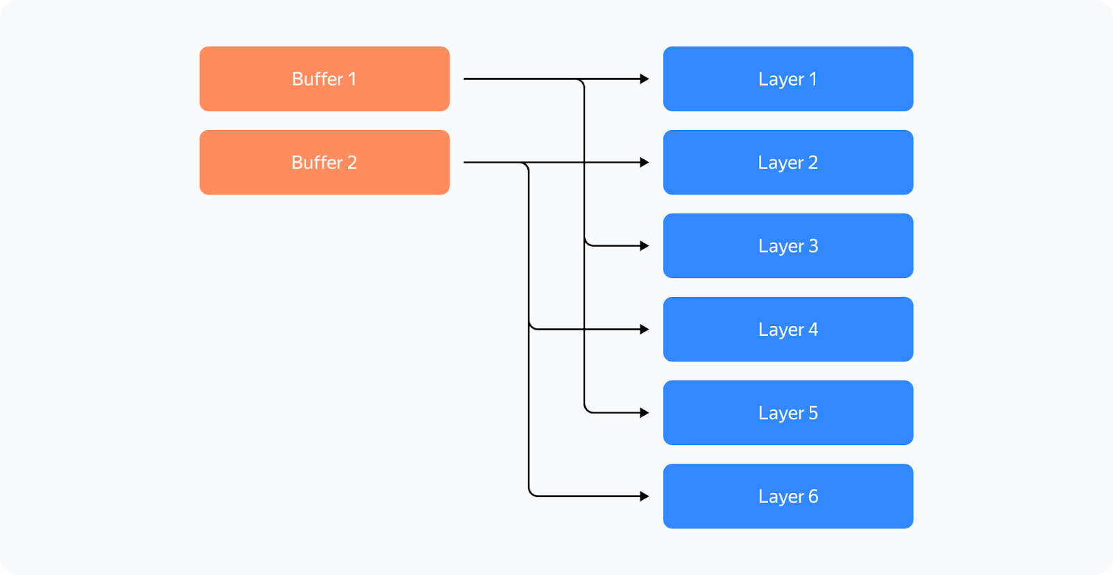
This way, the weights from different layers are stored in the same memory. If the layers have the same structure, they’ll always be identical! What’s important is to ensure that when you need layer X, the buffer has the weights for layer X. All parameters will be stored in the corresponding memory chunk in the buffer:

Other than that, the new method is similar to FSDP. Here’s what we’ll need:

• Buffers to store shards and gradients in fp32 for the optimizer (because of mixed precision).

• A buffer to store the weight shard in half precision (bf16 in our case).

Now we need to set up communications so that:

1. The forward/backward pass on the layer doesn’t start until the weights of that layer are collected in its buffer.

2. Before the forward/backward pass on a certain layer is completed, we don’t collect another layer in this layer’s buffer.

3. The backward pass on the layer doesn’t start until the reduce_scatter operation on the previous layer that uses the same gradient buffer is completed.

4. The reduce_scatter operation in the buffer doesn’t start until the backward pass on the corresponding layer is completed.

How do we achieve this setup?

Working with Streams

You can use CUDA streams to facilitate concurrent computations and communications.

How is the interaction between CPU and GPU organized in Torch and other frameworks? Kernels (functions executed on the GPU) are loaded from the CPU to the GPU in the order of execution. To avoid downtime due to the CPU, the kernels are loaded ahead of the computations and are executed asynchronously. Within a single stream, kernels are always executed in the order in which they were loaded to the CPU. If we want them to run in parallel, we need to load them to different streams. Note that if kernels in different streams use the same resources, they may fail to run in parallel (remember the “give-way effect” mentioned above) or their executions may be very slow.

To facilitate communication between streams, you can use the “event” primitive (event = torch.cuda.Event() in Torch). We can put an event into a stream (event.record(stream)), and then it’ll be appended to the end of the stream like a microkernel. We can wait for this event in another stream (event.wait(another_stream)), and then this stream will pause until the first stream reaches the event.

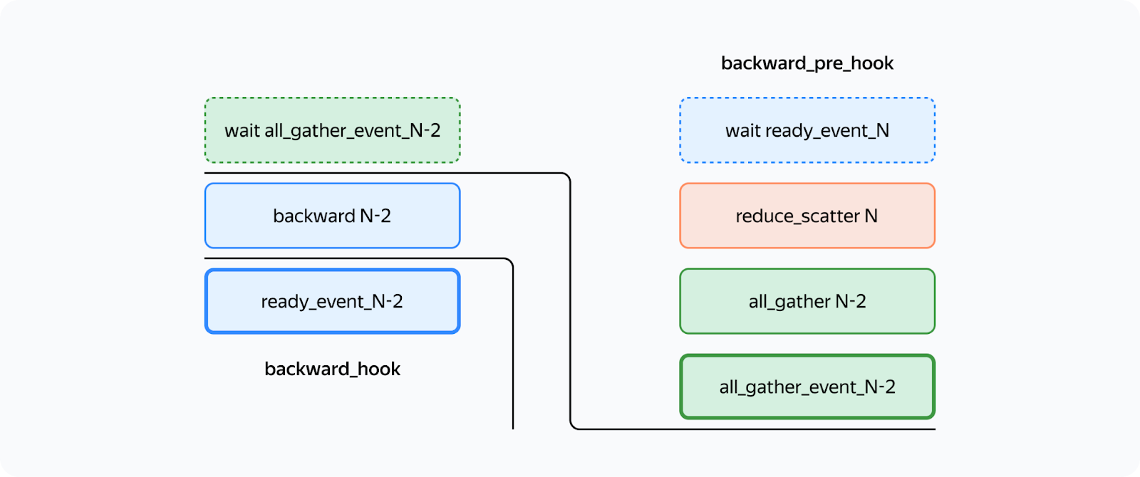
We only need two streams to implement this: a computation stream and a communication stream. This is how you can set up the execution to ensure that both conditions 1 and 2 (described above) are met:

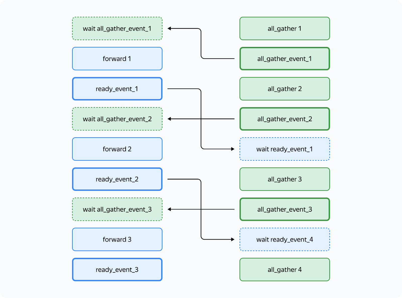
In the diagram, bold lines mark event.record() and dotted lines are used for event.wait(). As you can see, the forward pass on the third layer doesn’t start until the all_gather operation on that layer is completed (condition 1). Likewise, the all_gather operation on the third layer won’t start until the forward pass on the first layer that uses the same buffer is completed (condition 2). Since there are no cycles in this scheme, deadlock is impossible.

How can we implement this in Torch? You can use forward_pre_hook, code on the CPU executed before the forward pass, as well as forward_hood, which is executed after the pass:

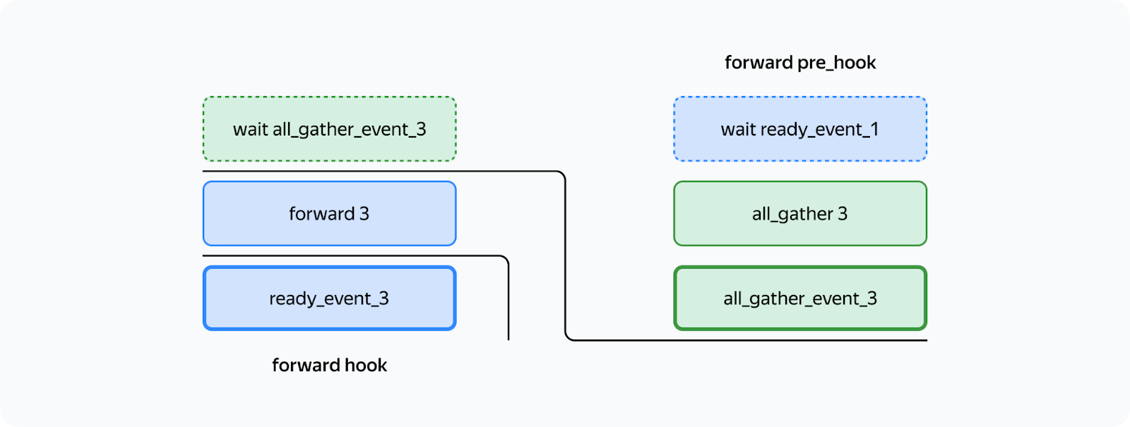
This way, all the preliminary operations are performed in forward_pre_hook. For more information about hooks, see the documentation.

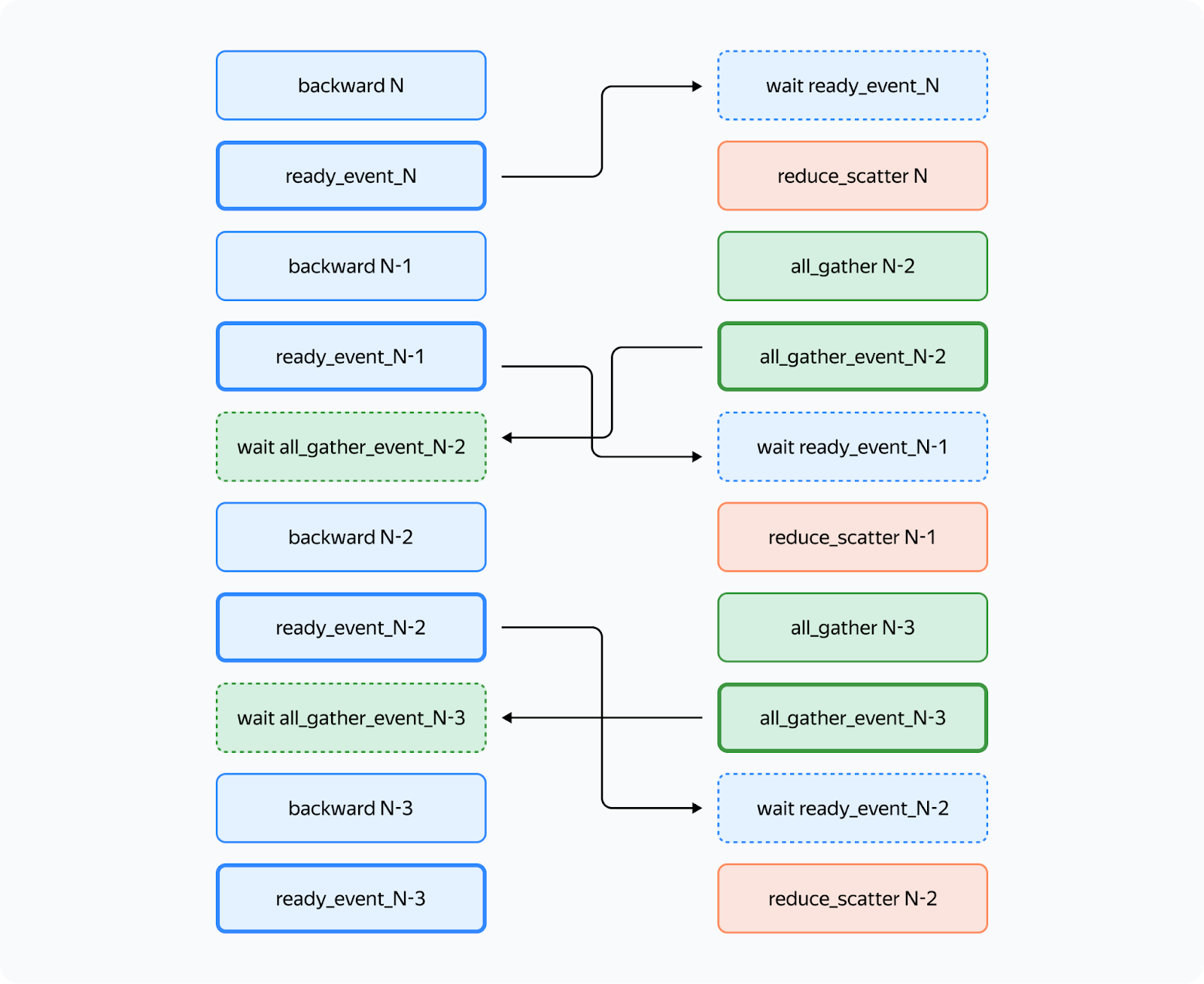
What’s different for the backward pass? Here, we’ll need to average gradients among processes:

We could try using backward_hook and backward_pre_hook in the same way we used forward_hook and forward_pre_hook: 

But there’s a catch: while backward_pre_hook works exactly as anticipated, backward_hook may behave unexpectedly:

— If the module input tensor has at least one tensor that doesn’t pass gradients (for example, the attention mask), backward_hook will run before the backward pass is executed.
— Even if all module input tensors pass gradients, there is no guarantee that backward_hook will run after the .grad of all tensors is computed.

So we aren’t satisfied with the initial implementation of backward_hook and need a more reliable solution.

Reliable backward_hook

Why isn’t backward_hook suitable? Let’s take a look at the gradient computation graph for relatively simple operations:

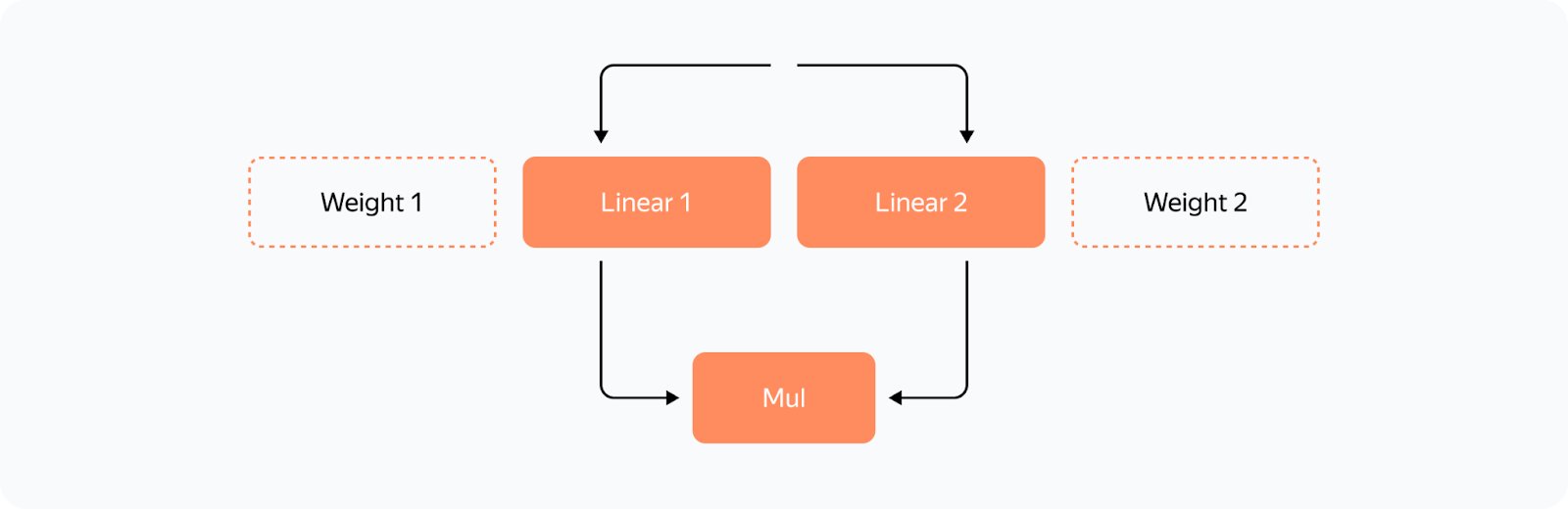
We apply two independent linear layers with Weight 1 and Weight 2 to the input and multiply their outputs.

The gradient computation graph will look like this:

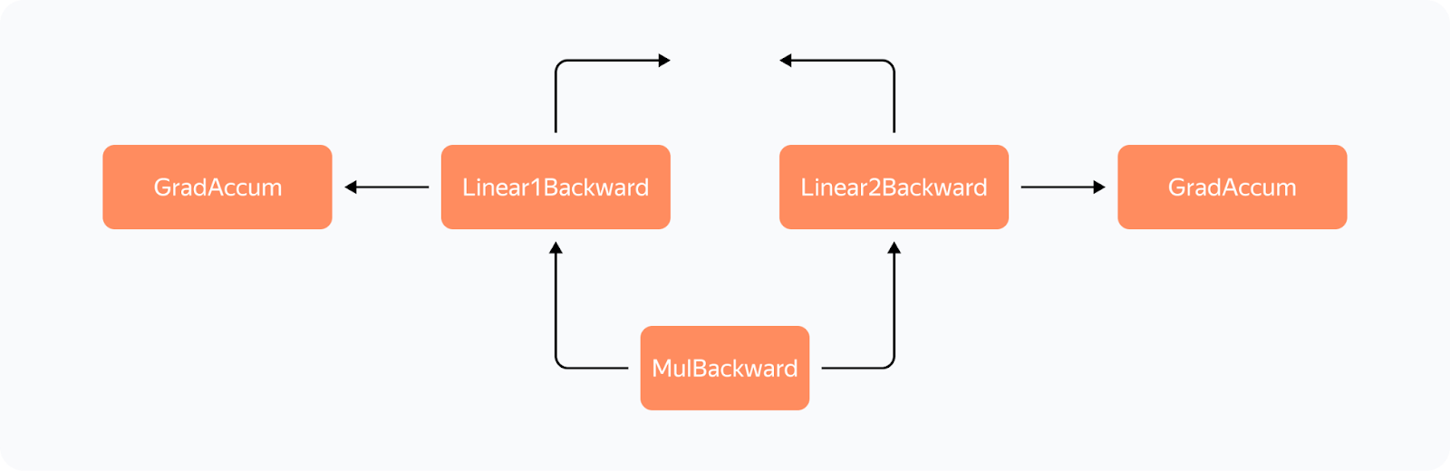
We can see that all operations have their *Backward nodes in this graph. For all weights in the graph, there’s a GradAccum node where the .grad of the parameter is updated. This parameter will then be used by YaFSDP to process the gradient.

Something to note here is that GradAccum is in the leaves of this graph. Curiously, Torch doesn’t guarantee the order of graph traversal. GradAccum of one of the weights can be executed after the gradient leaves this block. Graph execution in Torch is not deterministic and may vary from iteration to iteration.

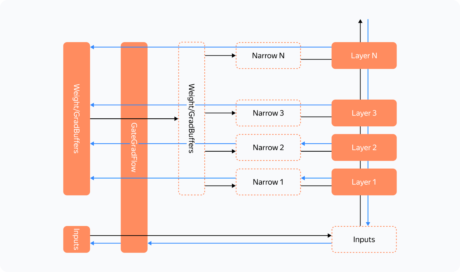
How do we ensure that the weight gradients are calculated before the backward pass on another layer starts? If we initiate reduce_scatter without making sure this condition is met, it’ll only process a part of the calculated gradients. Trying to work out a solution, we came up with the following schema:

Before each forward pass, the additional steps are carried out:

— We pass all inputs and weight buffers through GateGradFlow, a basic torch.autograd.Function that simply passes unchanged inputs and gradients through itself.

— In layers, we replace parameters with pseudoparameters stored in the weight buffer memory. To do this, we use our custom Narrow function. 

What happens on the backward pass: 

The gradient for parameters can be assigned in two ways:

— Normally, we’ll assign or add a gradient during the backward Narrow implementation, which is much earlier than when we get to the buffers’ GradAccum.
— We can write a custom function for the layers in which we’ll assign gradients without allocating an additional tensor to save memory. Then Narrow will receive “None” instead of a gradient and will do nothing.

With this, we can guarantee that:

— All gradients will be written to the gradient buffer before the backward GateGradFlow execution.
— Gradients won’t flow to inputs and then to “backward” of the next layers before the backward GateGradFlow is executed.

This means that the most suitable place for the backward_hook call is in the backward GateGradFlow! At that step, all weight gradients have been calculated and written while a backward pass on other layers hasn’t yet started. Now we have everything we need for concurrent communications and computations in the backward pass.

Overcoming the “Give-Way Effect’

The problem of the “give-way effect” is that several computation operations take place in the communication stream before reduce_scatter. These operations include copying gradients to a different buffer, “pre-divide” of gradients to prevent fp16 overflow (rarely used now), and others.

Here’s what we did:

— We added a separate processing for RMSNorm/LayerNorm. Because these should be processed a little differently in the optimizer, it makes sense to put them into a separate group. There aren’t many such weights, so we collect them once at the start of an iteration and average the gradients at the very end. This eliminated duplicate operations in the “give-way effect”.

— Since there’s no risk of overflow with reduce_scatter in bf16 or fp32, we replaced “pre-divide” with “post-divide”, moving the operation to the very end of the backward pass.

As a result, we got rid of the “give-way effect”, which greatly reduced the downtime in computations:

Restrictions

The YaFSDP method optimizes memory consumption and allows for a significant gain in performance. However, it also has some restrictions:

— You can reach peak performance only if the layers are called so that their corresponding buffers alternate.
— We explicitly take into account that, from the optimizer’s point of view, there can be only one group of weights with a large number of parameters.

Test Results

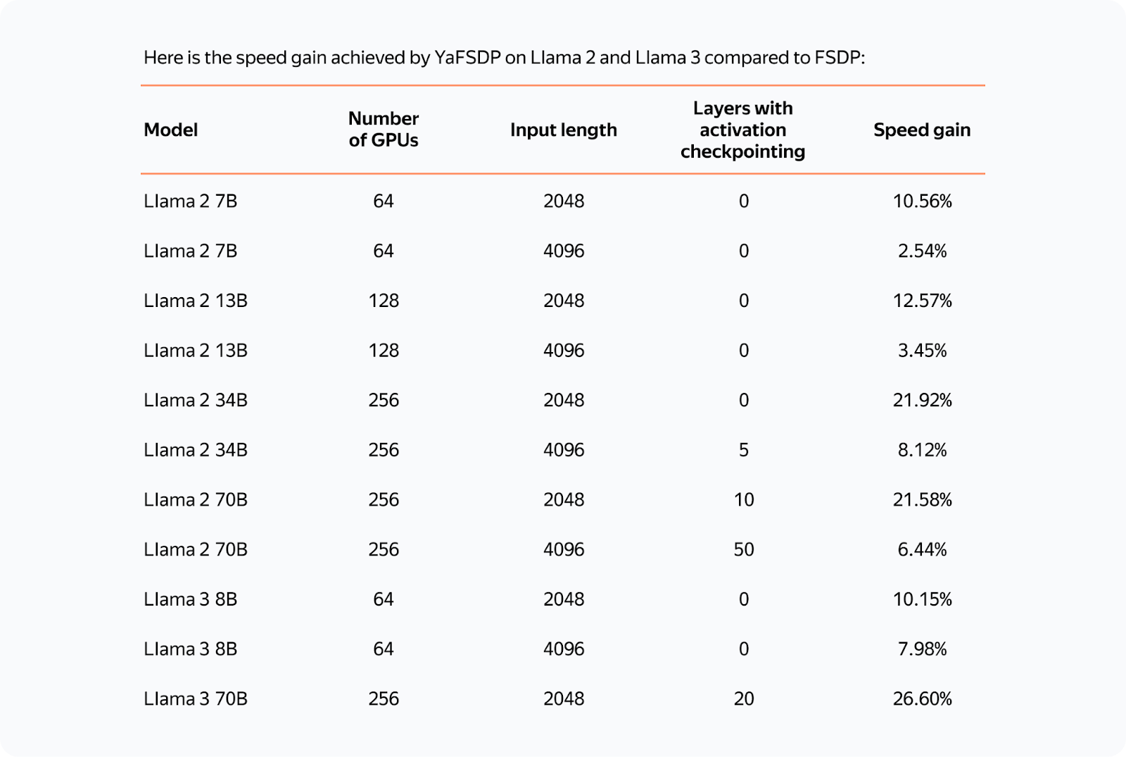
The resulting speed gain in small-batch scenarios exceeds 20%, making YaFSDP a useful tool for fine-turning models.

In Yandex’s pre-trainings, the implementation of YaFSDP along with other memory optimization strategies resulted in a speed gain of 45%.

Now that YaFSDP is open-source, you can check it out and tell us what you think! Please share comments about your experience, and we’d be happy to consider possible pull requests.

*This post was written by Mikhail Khrushchev, the leader of the YandexGPT pre-training team, and originally published here. We thank Yandex for their insights and ongoing support of TheSequence.